5 min to read
Linear Regression with python

There are two types of supervised machine learning algorithms which are regression and classification. Linear regression is a machine learning algorithm. Most of the time, it is used to find out the relationship between input variables (x) and output variables (y). If you plot x on the x-axis and the y on the y-axis, linear regression is the line that best fit the data points as show below. This article isn’t about explanation of linear regression. Others might have better explanations than me.
Simple linear regression
Let’s start with the dataset. For this simple task, we’re going to predict the student’s score based on hours of study, instead of using the popular Boston house price task. The information in this dataset is not much to say, it only contains the scores and the hours of study. Obviously, you can make it up your own.
Before we dive into coding, you might want to import some neccessary libraries.
import pandas as pd
import numpy as np
import matplotlib.pyplot as plt
from sklearn.model_selection import train_test_split
from sklearn.linear_model import LinearRegression
from sklearn import metrics
We will start with a simple way of implementing linear regression
numpy. A powerful math library to do vectorized numerical calculations.matplotlibThis will helps you plot the graph to gain a better understandingpandasA library that helps you to read csv files.sklearnA package that implements multiple machine learning algorithms.
Let’s start by importing the dataset.
dataset = pd.read_csv('student_scores.csv')
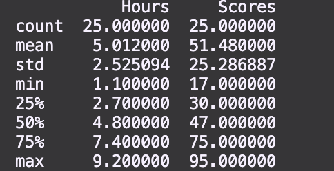
Then you might want to explore the dataset by using this describe() function.
dataset.describe()
You will be able to see something like this
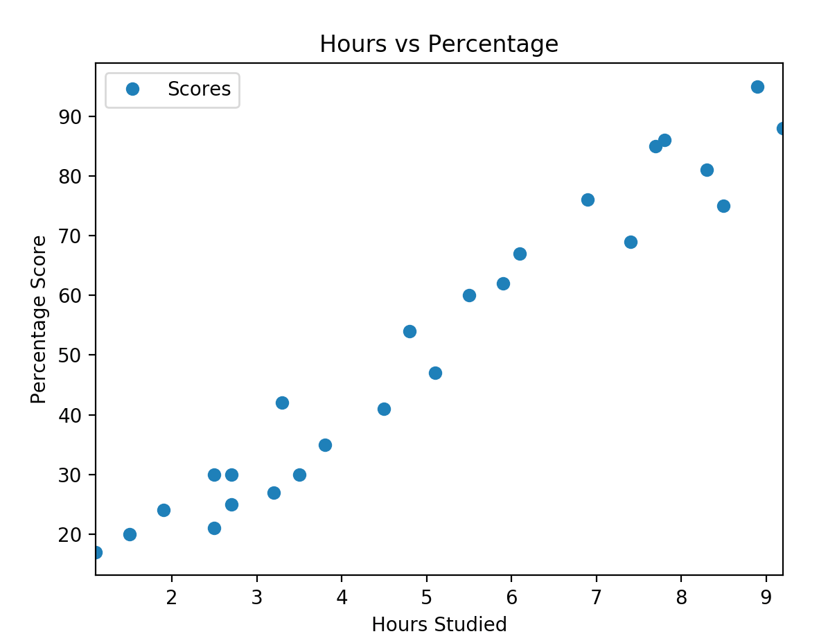
Finally, you might want to to plot your data using matplotlib so you can find the relationship between data points
dataset.plot(x='Hours', y='Scores', style='o')
plt.title('Hours vs Percentage')
plt.xlabel('Hours Studied')
plt.ylabel('Percentage Score')
plt.show()
The result will be displayed like this:
Our next step is to divide the data into “attributes” and “labels”. Attributes are the independent variables and labels are dependent variables whose values are to be predicted. In our dataset, we only have two columns, we want to predict the scores depending on the hours of study. Therefore our independent variables would be the hours of study (x) and the label will be the score which is stored in y variable.
X = dataset['Hours'].values.reshape(-1,1)
y = dataset['Scores'].values
Now you might want to split the 80% of the data into the training set, and 20% of the data will be used to test.
X_train, X_test, y_train, y_test = train_test_split(X, y, test_size=0.2, random_state=0)
After splitting the data into training and testing sets, it is now the time to train the algorithm. You will need to initialize LinearRegression class, and call the fit functions with our trained data.
regressor = LinearRegression()
regressor.fit(X_train, y_train)
After you train the dataset, you can start predict using predict() function and see how accurately the algorithm predicts the percentage score.
y_pred = regressor.predict(X_test)
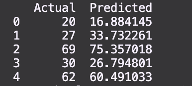
Next, you can compare the predicted values with the actual values.
df = pd.DataFrame({'Actual': y_test, 'Predicted': y_pred})
print(df)
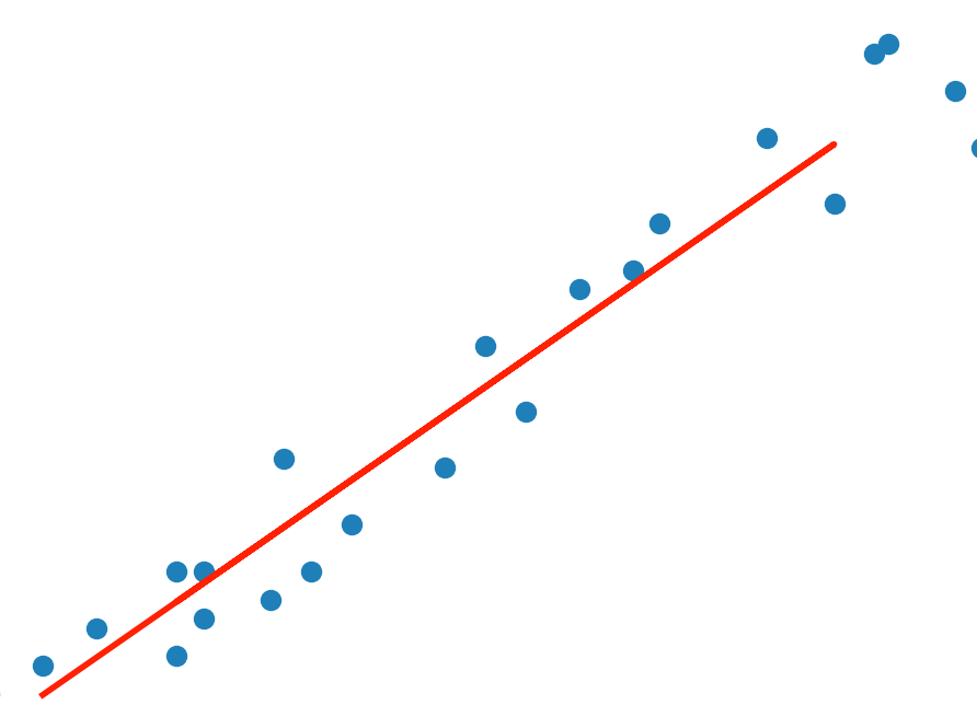
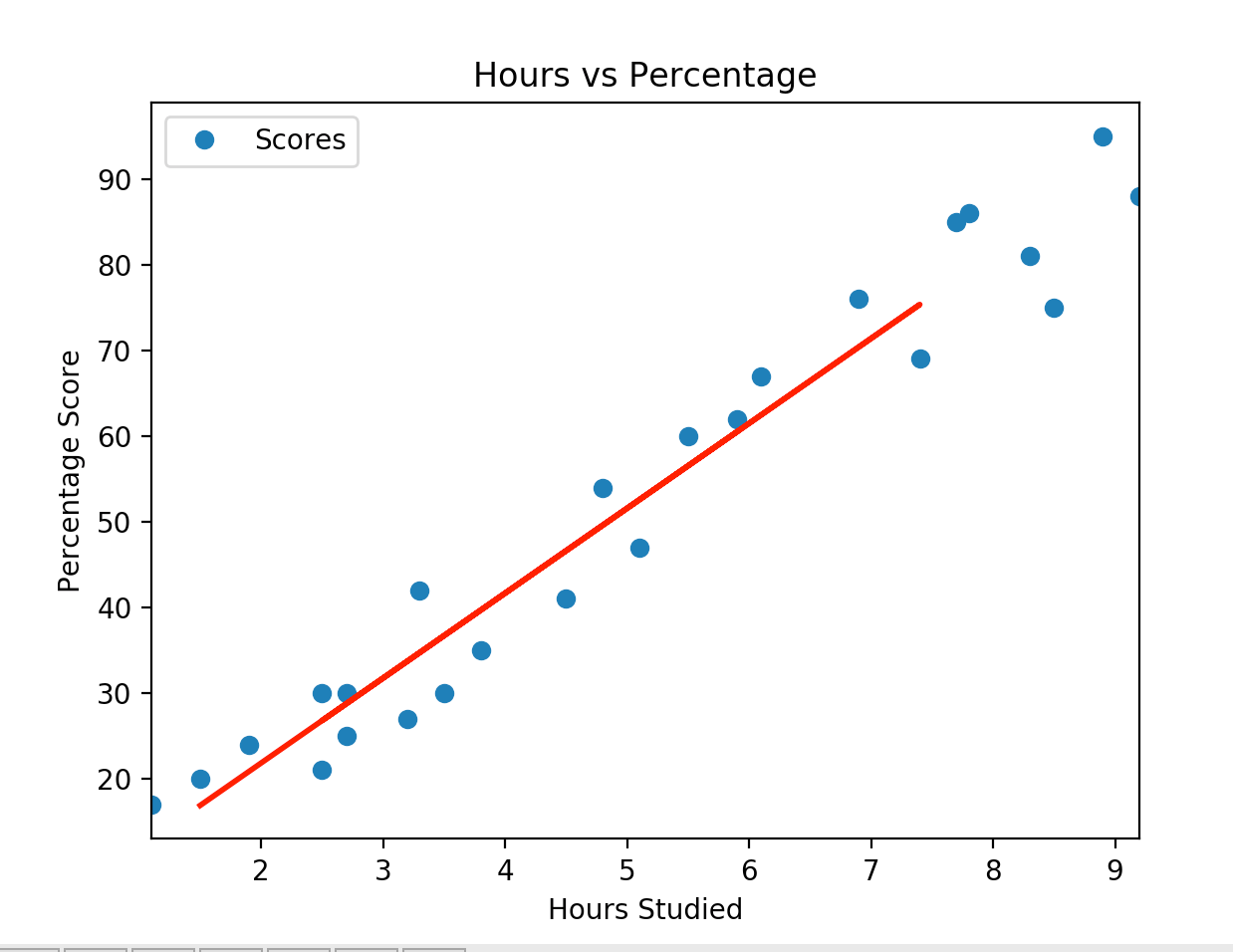
And, finally, plot our straight line
dataset.plot(x='Hours', y='Scores', style='o')
plt.plot(X_test, y_pred, color='red', linewidth=2)
plt.title('Hours vs Percentage')
plt.xlabel('Hours Studied')
plt.ylabel('Percentage Score')
plt.show()
How do we know how well the algorithm performs?
Before answer the questions, let’s try to understand what was going on here. How the linear regression class works under the hood.
We need to evaluate the performance of the algorithms so we can adjust and see if we can improve it. This process is called Cost function. There are 3 metrics commonly used to evaluate.
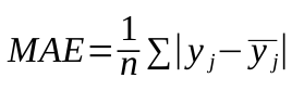
Mean Absolute Error (MAE)
The mean of the absolute value of the error
Mean Squared Error (MSE)
The mean of the squared error
Root Mean Squared Error (RMSE)
The square root of the mean of the squared errors:
Let’s implement the Mean Squared Error as our cost function
def compute_cost(X, y, param):
    n = len(y)
    h = X @ param
    return np.sum((h-y) ** 2)/(2*n)
The h variable represents our hypothesis function


Comments